Poster
Client Context
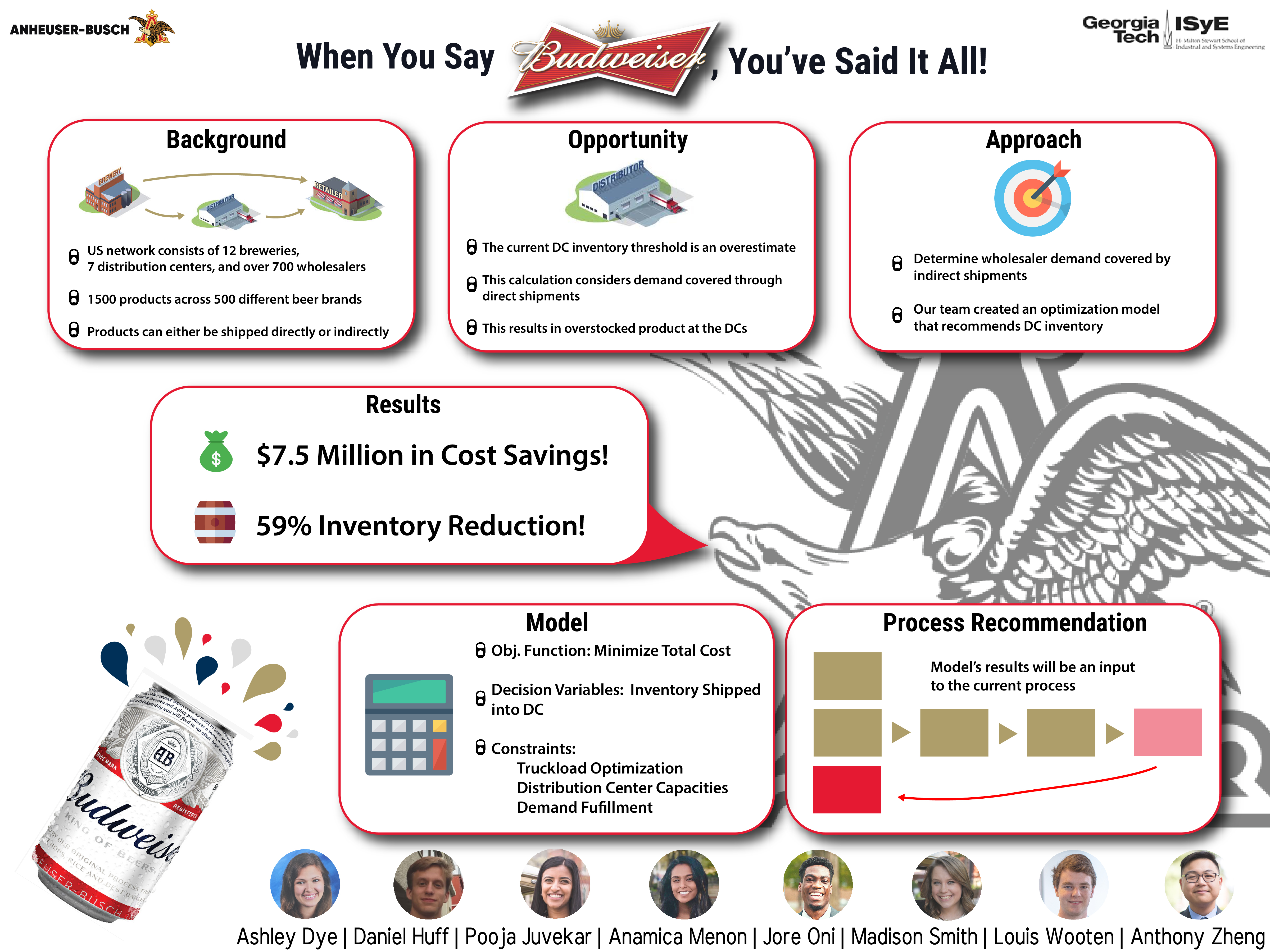
Anheuser-Busch (AB) is headquartered in St. Louis, Missouri, and is the largest brewing company in the world. AB dominates just under half of the American beer market with an arsenal of over 1,500 product containers (PDCNs, AB’s unique identifier for products) making up over 500 different beer brands. In the US, AB has a complex supply chain network that consists of 12 breweries, 7 distribution centers (DCs), 700+ wholesalers (WSLRs, who sell AB products to retailers). The senior design team worked with AB’s Supply Network Planning (SNP) team who controls the allocation of inventory to each WLSR to meet its forecasted demand.
Due to Prohibition era laws, AB cannot sell products directly to retailers and considers WSLRs their final customers. Breweries have two options on how to ship the product to a WSLR: directly from the brewery to the WSLR, or indirectly from the brewery to a DC, and then from the DC to a WSLR. Every WSLR has a DC in close proximity which is its designated “home location” DC. If a product is shipped indirectly, it will go through the WSLR’s home location. WSLRs become passive entities after forecasts are sent because the PDCN amount shipped and the lane, or shipping route, utilized to deliver the PDCNs are entirely decided by AB.
AB currently has an extensive process to calculate WSLR inventory through the use of multiple optimizers taking in two main inputs of AB’s long term inventory policies and the WLSR’s short term demand forecasts. This process outputs the inventory needed at each WSLR each week. AB calculates a DC inventory threshold by aggregating WSLR inventories by home location.
Project Objective
After understanding the current inventory calculation, the team wanted to look at the current DC performance by analyzing a detailed breakdown of total dumping/overage cost for each DC. The team observed, of the total dumped DC inventory in 2020, a significant portion was due to a lack of demand. Using this analysis of unnecessary cost due to overstocked product, it became clear that the current maximum DC inventory threshold calculation is an overestimate. This is because the summation of WSLR inventories by home location includes demand that will eventually be fulfilled via direct shipments from the brewery. Because this maximum threshold is so high, it does not constrain the DC volume shipped, so more product is being sent to the DCs than necessary, leading to overstocked product.
The project objective is to provide AB with a method of accurate DC inventory calculations to promote effective DC utilization.
Design Strategy
The approach to achieving the objective is to build an optimization model that determines what portion of WSLR demand will be covered by indirect shipments and then use this demand to determine DC inventory levels prior to the CONA optimizer being run. This approach is expected to result in a significant reduction of excess inventory held at the DCs. With this new optimal DC volume being an input into the CONA optimizer, the CONA output will have more accurate shipments.
The most important data input is a demand distribution for each DC-PDCN-month combination that is sampled into various scenarios to account for demand variability. To create this distribution, the WSLR demand fulfilled by indirect shipments was needed.
AB’s ABCD logic was utilized to determine the WSLR indirect shipment quantity. This logic designates volume thresholds that are compared to WSLR forecasts based on the WSLR’s home location and PDCN container type. The thresholds in order from highest to lowest are A, B, C, and D. For the model, just like in the current system, if the forecast is classified as an A or B, it will ship directly. If the forecast is classified as a C or D, it will ship indirectly. Since the focus of this project is on the DCs, only volume below the C and D thresholds were considered for DC demand. This created the indirect demand for each WSLR-PDCN-month combination, which was needed to create a DC demand distribution.
Data was inputted into the model by creating an object oriented program in Python to classify each data input by its type and creating a network of data to interact. Object oriented programming is used to structure a software program into simple, reusable pieces of code blueprints, called classes, which are used to create individual instances of objects. The model was then built in Python utilizing Pyomo with the Gurobi optimizer. Pyomo is a package used to help create optimization models, and the Gurobi optimizer is used to solve optimization models. There are 180,000+ decision variables and 19,000+ constraints in the model.
To validate the model, actual quantities of inventory sent to the DCs in 2019 were plugged into the model’s objective function, to compare to the actual 2019 DC cost described in Appendix 7. The model’s cost had a 4.09% difference compared to the actual cost. Therefore, it was confirmed that the objective function is accurate in modeling cost. The calculations of actual VLC and handling costs in 2019 vs. the model’s cost output using 2019 actuals by DC can be found in Appendix 7. The volume shipped into the DCs was consistent between actuals and validation (5,199,839 barrels).
Deliverables
t maintains the ability to meet AB’s service levels while minimizing cost. Service level is AB’s measure of system performance. A 99.7% service level, which is desired by AB, is a 99.7% expected probability of not hitting a stockout.
The objective function of the model is to minimize the total expected DC cost. After consultation with AB, four types of costs were identified as the main drivers of DC costs. These were variable logistics cost (VLC), handling cost, overage cost, and underage cost.
The model’s main decision variables are the recommended number of barrels of each PDCN to ship to each DC in each month. This volume quantity is converted into other units of measure of pallets, trucks, and cases to output other decision variables to accurately calculate the different costs stated above.
The model output is in the form of an Excel file that can be fed into the CONA optimizer. This Excel file includes the month-DC-PDCN volume needed for the horizon that the forecast data projects. This will allow AB to use the model for long and short term projections. AB may also use the output of the model to compare against the projected volumes to be sent to the DCs after the CONA and WSNP optimizers have been run. The SNP team will be able to use this as a sanity check to ensure that unnecessary volume is not being sent to the DCs.
AB can also utilize this model for future analysis. Since volume thresholds from ABCD logic are used to determine if a shipment should be indirect or direct, AB has the opportunity to modify these thresholds to test different levels. Another potential implementation of the model’s output would be in the form of a Power BI dashboard, which would help visualize the inventory recommendations by PDCN and Container type. Power BI was selected, as it is AB’s primary business analytics visualization program.
Project Information
Student Team
Dye, Ashley; Huff, Daniel; Juvekar, Pooja; Menon, Anamica; Oni, Jore; Smith, Madison; Wooten, Louis; Zheng, Anthony
Faculty Advisor

Faculty Evaluator